NeuralMath

Activation functions

The implementation begins with the two nonlinearities used by the network. ReLU acts in the hidden layer; the sigmoid maps the final score to the interval between 0 and 1.

def relu(s):
    return np.maximum(0, s)

def relu_derivative(s):
    return (s > 0).astype(float)

def sigmoid(s):
    return 1 / (1 + np.exp(-s))

Building a broad synthetic data set

We use mass and diameter as two physical features. The data are synthetic, but the values remain within plausible ranges for the teaching example. A smooth reference curve is used only to generate a nontrivial geometry; the network never receives that curve.

def base_boundary(m):
    return (
        6.68
        + 0.74 * np.exp(-((m - 155) / 20) ** 2)
        + 1.50 / (1 + np.exp(-(m - 202) / 5))
    )

X_train = np.vstack([apple_1, apple_2, orange_1, orange_2])
y_train = np.array([1.0] * 32 + [0.0] * 32)

Standardizing the inputs

Mass and diameter live on different numerical scales. The mean and standard deviation are computed only from the training set and then used consistently throughout the experiment.

mean = X_train.mean(axis=0)
std = X_train.std(axis=0)
Xn = (X_train - mean) / std

Initializing a 2–12–1 network

The model has two inputs, twelve ReLU hidden neurons, and one sigmoid output. This gives 49 trainable parameters while remaining small enough to inspect line by line.

rng = np.random.default_rng(42)
W1 = 0.1 * rng.standard_normal((12, 2))
b1 = np.zeros(12)
W2 = 0.1 * rng.standard_normal(12)
b2 = 0.0

Forward propagation

A prediction is just a sequence of affine transformations and activation functions. These four lines are the computational core of inference.

z1 = W1 @ x + b1
h = relu(z1)
z2 = W2 @ h + b2
y_hat = sigmoid(z2)

Backpropagation

The derivatives are written explicitly. There is no automatic differentiation: the chain rule appears directly in the code, which is the main pedagogical point of the example.

delta2 = (y_hat - target) * y_hat * (1 - y_hat)
dW2 = delta2 * h
db2 = delta2

delta1 = (delta2 * W2) * relu_derivative(z1)
dW1 = np.outer(delta1, x)
db1 = delta1

Stochastic gradient descent

At every epoch the examples are shuffled, and the parameters are updated after each observation. The procedure repeatedly uses the gradients computed above to reduce the loss.

for epoch in range(n_epochs):
    for i in rng.permutation(len(Xn)):
        # forward pass and backpropagation
        W1 -= learning_rate * dW1
        b1 -= learning_rate * db1
        W2 -= learning_rate * dW2
        b2 -= learning_rate * db2

What the training produces

With the fixed random seed and hyperparameters used here, the small network classifies all 64 training examples and all 8 illustrative test examples according to the labels defined for the synthetic experiment.

Final mean loss: 0.0001785644
Training accuracy: 1.0000
Illustrative test accuracy: 1.0000

Test outputs:
[121.0, 7.20] -> 0.999927 -> apple
[135.0, 7.45] -> 0.999900 -> apple
[152.0, 7.75] -> 0.999780 -> apple
[171.0, 7.32] -> 0.986972 -> apple
[121.0, 6.28] -> 0.000019 -> orange
[152.0, 6.86] -> 0.000009 -> orange
[189.0, 6.48] -> 0.000028 -> orange
[208.0, 7.55] -> 0.014957 -> orange

Drawing the learned decision boundary

After training, the network is evaluated on a dense grid. The level y-hat = 0.5 becomes the learned decision boundary, revealing the nonlinear geometry constructed by the hidden layer.

masses = np.linspace(116, 214, 500)
diameters = np.linspace(6.0, 8.85, 500)
M, D = np.meshgrid(masses, diameters)
grid = np.column_stack([M.ravel(), D.ravel()])
P = predict(grid, mean, std, W1, b1, W2, b2).reshape(M.shape)

ax.contour(M, D, P, levels=[0.5], linewidths=2.2)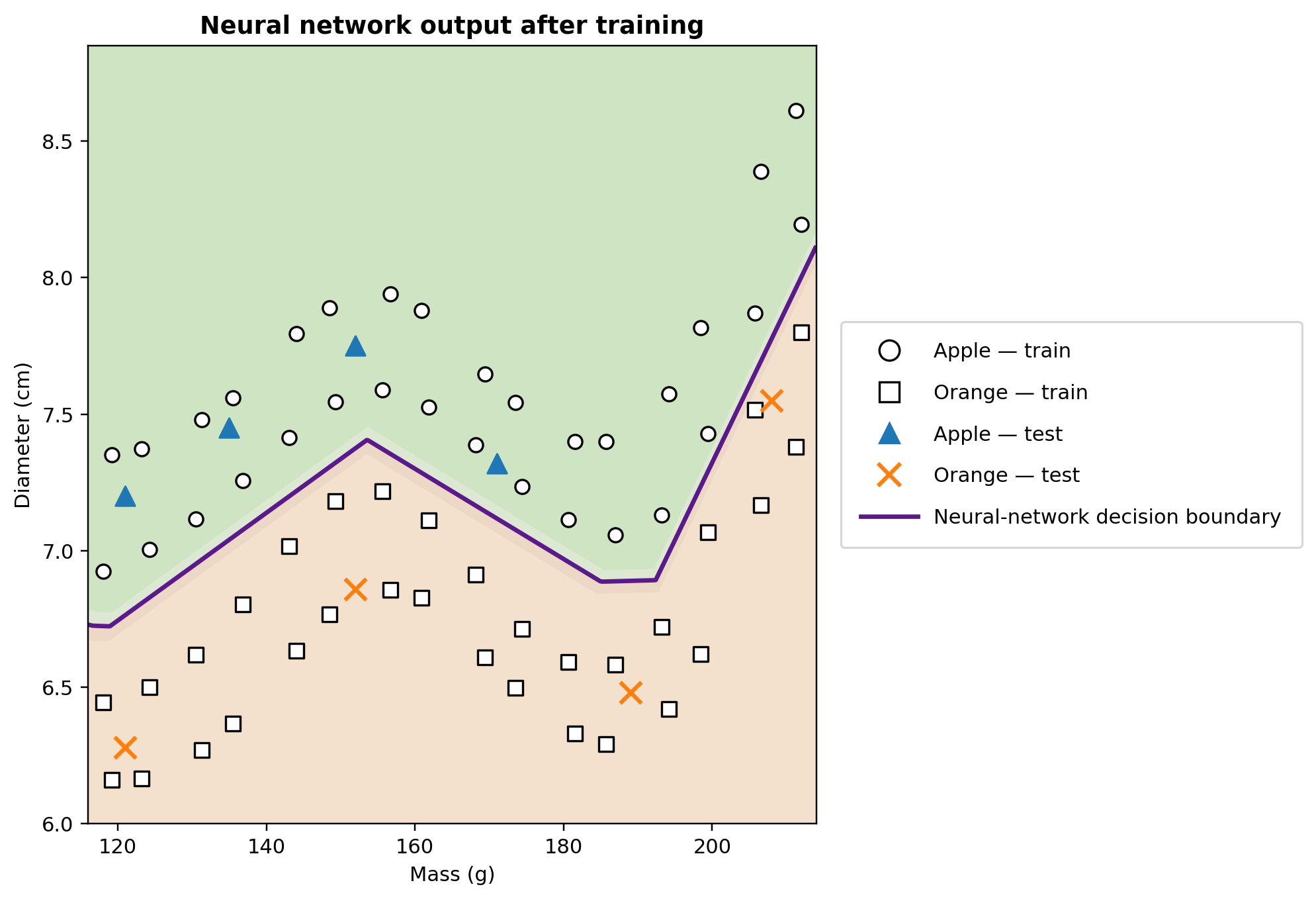

Full resources

The complete scripts, notebooks, and reproducible outputs are available below. The code shown on every language edition uses the same canonical English identifiers so the executable source never diverges across translations.

Python sourceGitHub repositoryGoogle ColabFigure (PDF)

Future extensions

NeuralMath is designed to grow as a sequence of computational examples rather than as a collection of disconnected pages. Planned extensions include training dynamics, visualizing hidden-neuron contributions, gradient checking, multiclass softmax classification, deeper networks, and small browser-based interactive experiments.

About the author

Americo Cunha Jr is a computational scientist, researcher at the Brazilian National Laboratory for Scientific Computing (LNCC), and associate professor at the State University of Rio de Janeiro (UERJ). His research lies at the intersection of nonlinear dynamics, mathematical and computational modeling, uncertainty quantification, inverse problems, and artificial intelligence/scientific machine learning. He received the 2023 ABMEC Young Scientist Award and is active in international editorial and scientific collaborations.

americocunha.orgORCIDGoogle Scholar

License

Unless otherwise stated, the explanatory website text and original website figures are made available under the Creative Commons Attribution 4.0 International license (CC BY 4.0). The pedagogical PDF may be subject to the license of its journal version. Source code is distributed separately and should carry its own software license.